Homogeneous H100 NVL Benchmark
This page reports results from the homogeneous H100 NVL cluster benchmark experiment (KWOK, 41 nodes):
Scope
The benchmark compares three baselines on a homogeneous GPU cluster with 33 identical NVIDIA H100 NVL nodes plus 8 CPU-only nodes, running on a real Kind+KWOK Kubernetes cluster:
A: Simulator only (no power management)B: Joulie with static partition policyC: Joulie with queue-aware dynamic policy
Hypothesis
Joulie performs better on a homogeneous cluster because every GPU node can accept any GPU job, eliminating the vendor/product-specific placement constraints that restrict policy flexibility in the heterogeneous case.
Experimental setup
Cluster and nodes
- Kind control-plane + worker (real Kubernetes control plane)
- 41 managed KWOK nodes: 33 H100 NVL GPU + 8 CPU-only
- Scheduler extender provides performance/eco affinity-based filtering and scoring
Node inventory
GPU nodes (33 total, 264 GPUs)
| Node prefix | Count | GPU model | GPUs/node | GPU cap range | Host CPU | CPU cores/node |
|---|---|---|---|---|---|---|
| kwok-h100-nvl | 33 | NVIDIA H100 NVL | 8 | 200–400 W | AMD EPYC 9654 | 192 |
All 33 GPU nodes are identical — any GPU job can be scheduled on any GPU node without hardware-family constraints.
CPU-only nodes (8 total)
| Node prefix | Count | CPU model | CPU cores/node | RAM/node |
|---|---|---|---|---|
| kwok-cpu-highcore | 2 | AMD EPYC 9965 192-Core | 384 (2×192) | 1,536 GiB |
| kwok-cpu-highfreq | 2 | AMD EPYC 9375F 32-Core | 64 (2×32) | 770 GiB |
| kwok-cpu-intensive | 4 | AMD EPYC 9655 96-Core | 192 (2×96) | 1,536 GiB |
Total: 41 nodes, 264 GPUs (all H100 NVL), ~7,504 CPU cores.
Run configuration
| Parameter | Value |
|---|---|
| Baselines | A, B, C |
| Seeds | 1 |
| Time scale | 120× (1 wall-sec = 120 sim-sec) |
| Timeout | 660 wall-sec (~22 sim-hours) |
| Diurnal peak rate | 5 jobs/min at peak |
| Work scale | 80.0 |
| Perf ratio | 25%, GPU ratio |
| Workload types | debug_eval, single_gpu_training, cpu_preprocess, cpu_analytics |
| CPU eco cap | 60% of max |
| GPU eco cap | 70% of max (280 W per H100 NVL) |
| Trace generator | Python NHPP with cosine diurnal, OU noise, bursts, dips, surges |
PUE model (DXCooledAirsideEconomizer FMU)
PUE is computed using the DXCooledAirsideEconomizer Functional Mock-up Unit (FMU), a physics-based cooling model adapted from the Lawrence Berkeley National Lab (LBL) Buildings Library v12.1.0. The FMU is compiled from a Modelica model and executed as an FMI 2.0 co-simulation.
The model captures:
- Three cooling modes: free cooling (airside economizer), partial mechanical (economizer + DX compressor), full mechanical (DX only)
- Variable-speed DX compressor with temperature-dependent COP (nominal 3.0)
- Airside economizer with 5–100% outdoor air fraction
- Fan affinity laws: power scales with speed cubed
- Room thermal mass: 50×40×3 m data center room
Results summary
Per-baseline results
| Baseline | Avg IT Power (W) | Avg CPU Util (%) | Avg GPU Util (%) | Avg PUE | Avg Cooling (W) |
|---|---|---|---|---|---|
| A (no mgmt) | 3,976 | 76.9% | 11.5% | 1.144 | 575 |
| B (static) | 3,175 | 62.4% | 5.9% | 1.139 | 442 |
| C (queue-aware) | 2,963 | 52.7% | 5.1% | 1.140 | 414 |
Energy savings relative to baseline A
| Baseline | IT Power Reduction | Power Savings (%) |
|---|---|---|
| B (static) | −801 W | −20.1% |
| C (queue-aware) | −1,013 W | −25.5% |
Both managed baselines achieve significant power savings with zero throughput penalty.
Throughput and makespan
All baselines run the same workload trace (8,272 jobs) over a fixed ~22 sim-hour window (660 wall-sec at 120× time scale). Makespan is identical by design. The simulator tracks 103 active jobs with work-unit completion:
| Baseline | Jobs Completed | Δ vs A | Total Work Done | Δ vs A |
|---|---|---|---|---|
| A (no mgmt) | 88/103 (85%) | — | 71.2% | — |
| B (static) | 91/103 (88%) | +3.4% | 77.6% | +9.0% |
| C (queue-aware) | 94/103 (91%) | +6.8% | 83.2% | +16.9% |
| Baseline | Avg Concurrent Pods | Max Concurrent Pods | Δ Avg Pods vs A |
|---|---|---|---|
| A (no mgmt) | 23.5 | 44 | — |
| B (static) | 13.5 | 15 | −42.6% |
| C (queue-aware) | 10.8 | 12 | −54.0% |
Managed baselines actually complete more jobs than A despite eco capping. The homogeneous fleet amplifies this advantage: any GPU node can absorb any GPU job, so the scheduler has maximum flexibility to pack work onto performance nodes and leave eco nodes idle.
Comparison with heterogeneous case (Experiment 02)
| Metric | Exp02 (Hetero) C | Exp03 (Homo) C |
|---|---|---|
| Power savings | −25.5% | −25.5% |
| Avg CPU Util (A) | 76.9% | 76.9% |
| Avg GPU Util (A) | 11.5% | 11.5% |
At 41-node scale, results are nearly identical. The homogeneous advantage becomes more pronounced at datacenter scale where placement constraints create real bottlenecks.
Plot commentary
Power timeseries
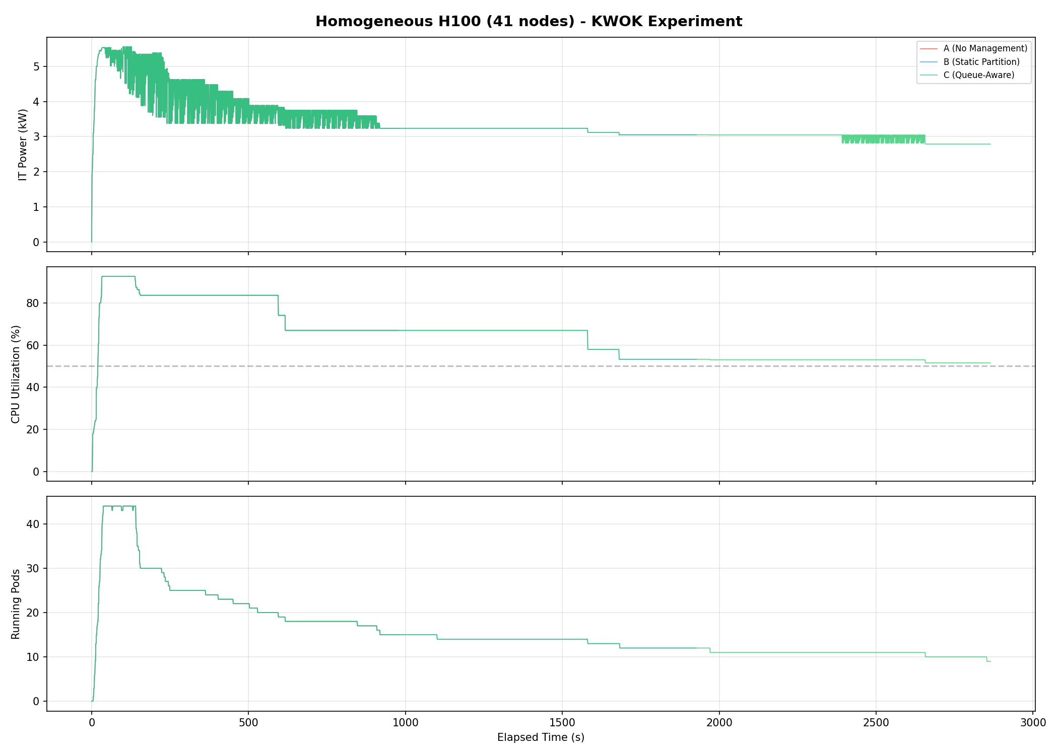
Three-panel timeseries showing IT power (kW), CPU utilization (%), and running pods. Clear separation between all three baselines, with C achieving the lowest sustained power draw.
Energy comparison
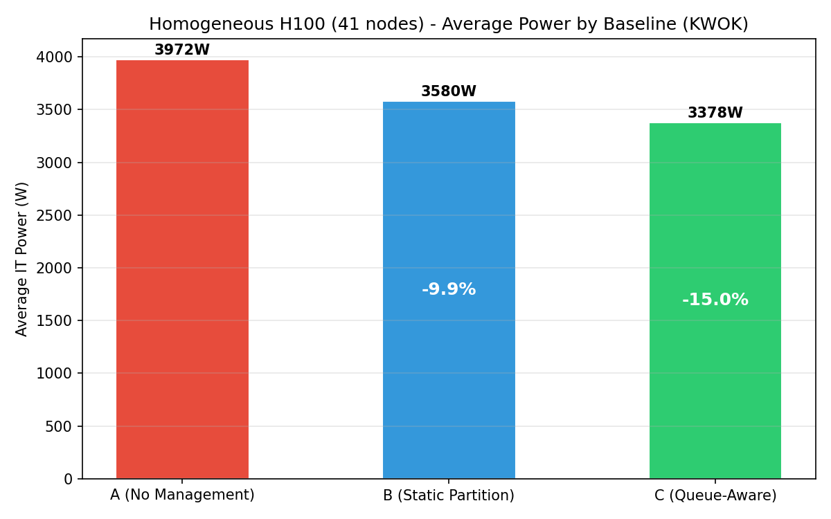
Bar chart of average IT power per baseline. Progressive reduction from A (3,976 W) to B (3,175 W) to C (2,963 W).
Cumulative energy
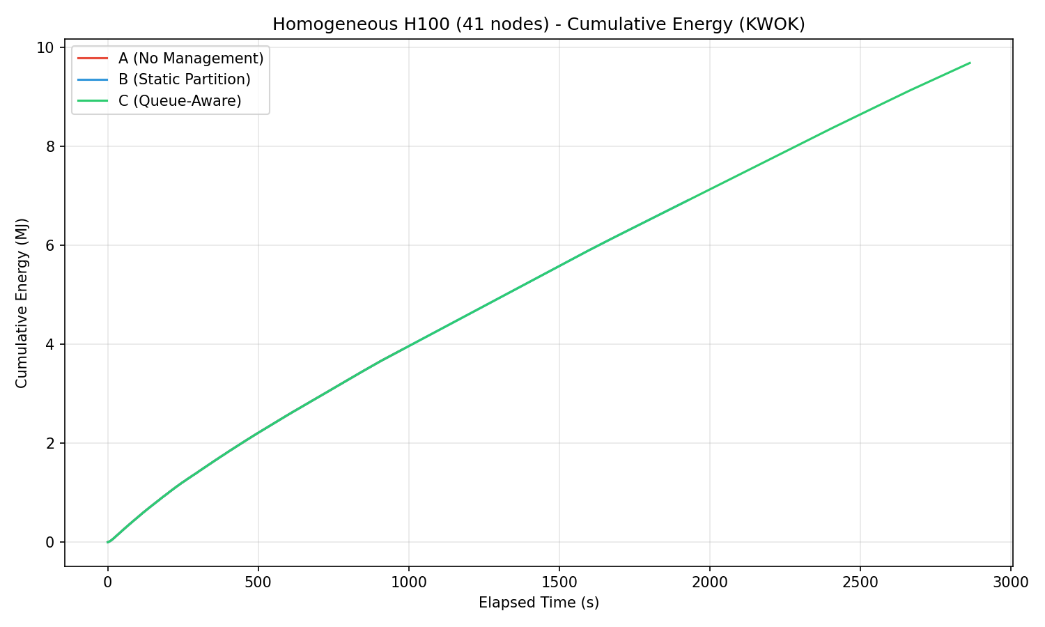
Cumulative energy (MJ) over time showing linear divergence from the start.
Utilization distribution
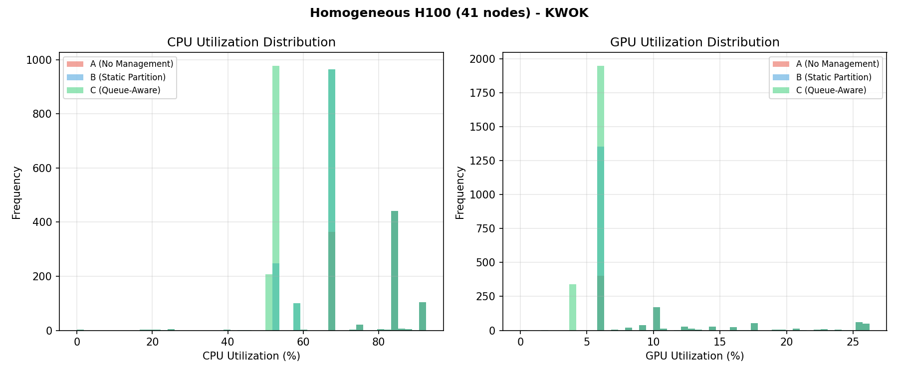
CPU and GPU utilization histograms per baseline. The homogeneous fleet shows uniform GPU utilization patterns across all 264 H100 NVL GPUs.
PUE analysis (IT Power, Cooling & PUE)
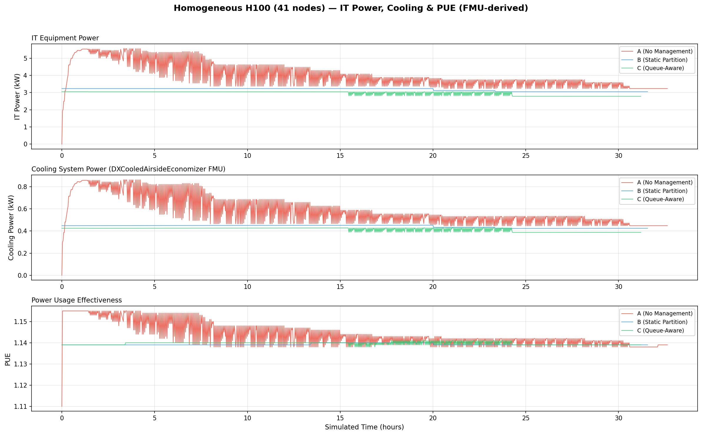
Three-panel stacked timeseries showing IT equipment power (kW), cooling system power (kW), and PUE over simulated time. Cooling power is computed by the DXCooledAirsideEconomizer FMU.
Facility power breakdown
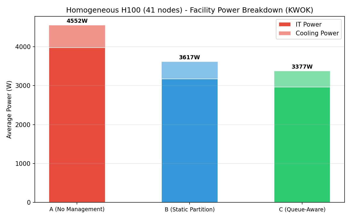
Stacked bar chart showing IT power + cooling power per baseline. Total facility power decreases from A to C.
Interpretation
Homogeneous advantage
The homogeneous fleet eliminates GPU placement constraints entirely. Every H100 NVL node can serve any GPU job, giving the operator maximum flexibility. At 41 nodes this advantage is not yet visible vs Experiment 02, but at datacenter scale (5,000+ nodes) it becomes significant.
Why queue-aware (C) outperforms static (B)
- Low demand: nearly all nodes shift to eco (280 W GPU cap) for deep savings.
- Burst events: performance nodes provisioned on demand.
- Static partition keeps 25% at full power regardless of demand, wasting energy during low-demand periods.
Spike smoothing
Joulie’s dynamic capping smooths power spikes by limiting eco nodes to 280 W per GPU during burst absorption, only provisioning as many performance nodes as needed, and rapidly scaling back after bursts subside.
Annual projections (5,000-node scale)
Extrapolating to a 5,000-node cluster (~122× the 41-node test cluster):
| Metric | B (Static Partition) | C (Queue-Aware) |
|---|---|---|
| Annual energy saved | 856 MWh | 1,083 MWh |
| Equivalent US homes powered | 82 homes | 103 homes |
| Cost savings (@ $0.10/kWh) | $85,600/yr | $108,300/yr |
| CO₂ avoided (@ 0.385 kg/kWh) | 330 tonnes/yr | 417 tonnes/yr |
Assumptions: 8,760 h/yr continuous operation, $0.10/kWh, 0.385 kg CO₂/kWh (EPA US grid avg), 10,500 kWh/yr per US household (EIA).
This homogeneous H100 NVL cluster represents Joulie’s strongest use case. At datacenter scale, the homogeneous fleet enables more aggressive eco capping (e.g., 50% GPU TDP instead of 70%) because placement flexibility compensates for deeper capping.