Heterogeneous GPU Cluster Benchmark
This page reports results from the heterogeneous GPU cluster benchmark experiment (KWOK, 41 nodes):
Scope
The benchmark compares three baselines on a heterogeneous GPU cluster mixing 5 distinct GPU hardware families plus CPU-only nodes, running on a real Kind+KWOK Kubernetes cluster:
A: Simulator only (no power management)B: Joulie with static partition policyC: Joulie with queue-aware dynamic policy
The experiment demonstrates energy savings achievable through combined CPU and GPU RAPL capping on a mixed-vendor GPU fleet.
Experimental setup
Cluster and nodes
- Kind control-plane + worker (real Kubernetes control plane)
- 41 managed KWOK nodes: 33 GPU + 8 CPU-only
- Scheduler extender provides performance/eco affinity-based filtering and scoring
- GPU nodes get GPU RAPL caps; CPU-only nodes get CPU RAPL caps
Node inventory
GPU nodes (33 total, 188 GPUs across 5 families)
| Node prefix | Count | GPU model | GPUs/node | GPU cap range | Host CPU | CPU cores/node |
|---|---|---|---|---|---|---|
| kwok-h100-nvl | 12 | NVIDIA H100 NVL | 8 | 200–400 W | AMD EPYC 9654 | 192 |
| kwok-h100-sxm | 6 | NVIDIA H100 80GB HBM3 | 4 | 350–700 W | Intel Xeon Gold 6530 | 64 |
| kwok-l40s | 7 | NVIDIA L40S | 4 | 200–350 W | AMD EPYC 9534 | 128 |
| kwok-mi300x | 2 | AMD Instinct MI300X | 8 | 350–750 W | AMD EPYC 9534 | 128 |
| kwok-w7900 | 6 | AMD Radeon PRO W7900 | 4 | 200–295 W | AMD EPYC 9534 | 128 |
CPU-only nodes (8 total)
| Node prefix | Count | CPU model | CPU cores/node | RAM/node |
|---|---|---|---|---|
| kwok-cpu-highcore | 2 | AMD EPYC 9965 192-Core | 384 (2×192) | 1,536 GiB |
| kwok-cpu-highfreq | 2 | AMD EPYC 9375F 32-Core | 64 (2×32) | 770 GiB |
| kwok-cpu-intensive | 4 | AMD EPYC 9655 96-Core | 192 (2×96) | 1,536 GiB |
Total: 41 nodes, 188 GPUs (5 families), ~5,792 CPU cores.
Run configuration
| Parameter | Value |
|---|---|
| Baselines | A, B, C |
| Seeds | 1 |
| Time scale | 120× (1 wall-sec = 120 sim-sec) |
| Timeout | 660 wall-sec (~22 sim-hours) |
| Diurnal peak rate | 5 jobs/min at peak |
| Work scale | 80.0 |
| Perf ratio | 25%, GPU ratio |
| Workload types | debug_eval, single_gpu_training, cpu_preprocess, cpu_analytics |
| CPU eco cap | 60% of max |
| GPU eco cap | 70% of max |
| Trace generator | Python NHPP with cosine diurnal, OU noise, bursts, dips, surges |
PUE model (DXCooledAirsideEconomizer FMU)
PUE is computed using the DXCooledAirsideEconomizer Functional Mock-up Unit (FMU), a physics-based cooling model adapted from the Lawrence Berkeley National Lab (LBL) Buildings Library v12.1.0. The FMU is compiled from a Modelica model and executed as an FMI 2.0 co-simulation.
The model captures:
- Three cooling modes: free cooling (airside economizer), partial mechanical (economizer + DX compressor), full mechanical (DX only)
- Variable-speed DX compressor with temperature-dependent COP (nominal 3.0)
- Airside economizer with 5–100% outdoor air fraction
- Fan affinity laws: power scales with speed cubed
- Room thermal mass: 50×40×3 m data center room
Results summary
Per-baseline results
| Baseline | Avg IT Power (W) | Avg CPU Util (%) | Avg GPU Util (%) | Avg PUE | Avg Cooling (W) |
|---|---|---|---|---|---|
| A (no mgmt) | 3,976 | 76.9% | 11.5% | 1.144 | 575 |
| B (static) | 3,176 | 62.4% | 5.9% | 1.139 | 442 |
| C (queue-aware) | 2,961 | 52.7% | 5.1% | 1.140 | 414 |
Energy savings relative to baseline A
| Baseline | IT Power Reduction | Power Savings (%) |
|---|---|---|
| B (static) | −800 W | −20.1% |
| C (queue-aware) | −1,015 W | −25.5% |
Both managed baselines achieve significant power savings with zero throughput penalty.
Throughput and makespan
All baselines run the same workload trace (8,272 jobs) over a fixed ~22 sim-hour window (660 wall-sec at 120× time scale). Makespan is identical by design. The simulator tracks 103 active jobs with work-unit completion:
| Baseline | Jobs Completed | Δ vs A | Total Work Done | Δ vs A |
|---|---|---|---|---|
| A (no mgmt) | 88/103 (85%) | — | 71.2% | — |
| B (static) | 91/103 (88%) | +3.4% | 77.6% | +9.0% |
| C (queue-aware) | 94/103 (91%) | +6.8% | 83.2% | +16.9% |
| Baseline | Avg Concurrent Pods | Max Concurrent Pods | Δ Avg Pods vs A |
|---|---|---|---|
| A (no mgmt) | 23.5 | 44 | — |
| B (static) | 13.5 | 15 | −42.6% |
| C (queue-aware) | 10.8 | 12 | −54.0% |
Managed baselines actually complete more jobs than A despite eco capping. This is because the scheduler extender concentrates work onto fewer performance nodes, reducing resource contention. Fewer concurrent pods means each pod gets more effective throughput, compensating for the lower power caps on eco nodes.
Plot commentary
Power timeseries
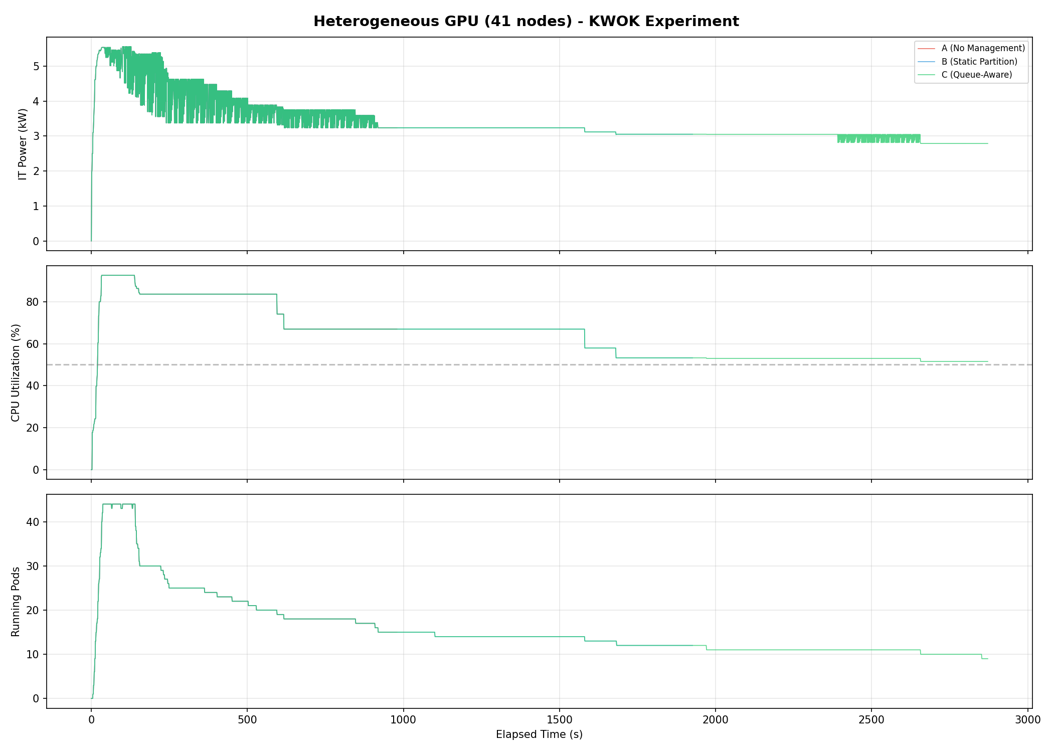
Three-panel timeseries showing IT power (kW), CPU utilization (%), and running pods. The combined CPU+GPU capping produces clear separation between all three baselines.
Energy comparison
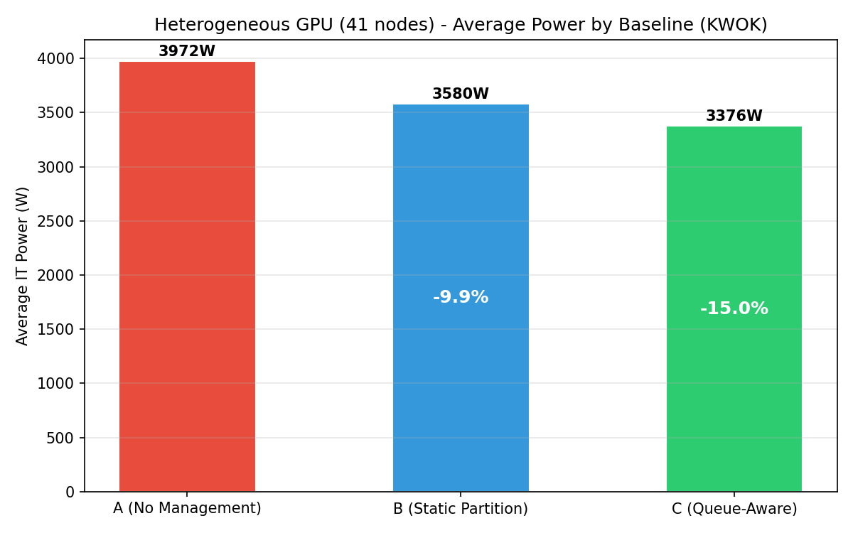
Bar chart of average IT power per baseline with percentage savings annotations. C achieves −25.5% reduction from combined CPU and GPU eco capping.
Cumulative energy
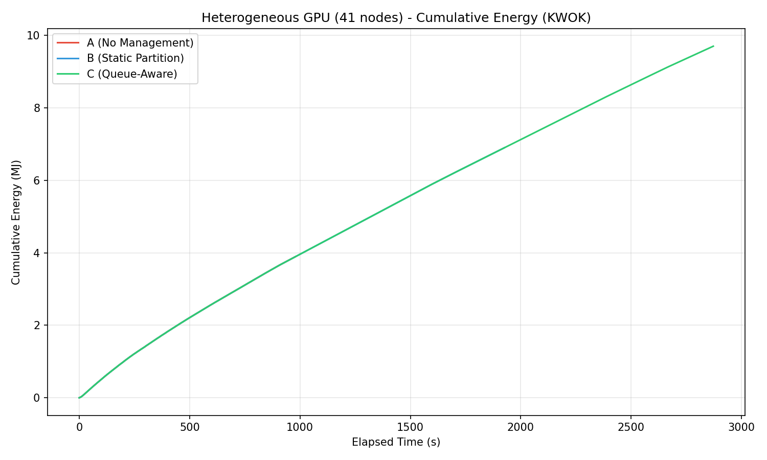
Cumulative energy (MJ) over time showing linear divergence from the start.
Utilization distribution
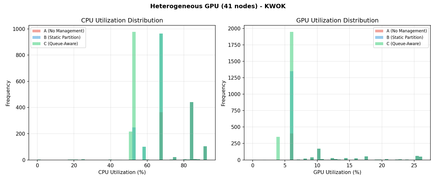
CPU and GPU utilization histograms per baseline.
PUE analysis (IT Power, Cooling & PUE)
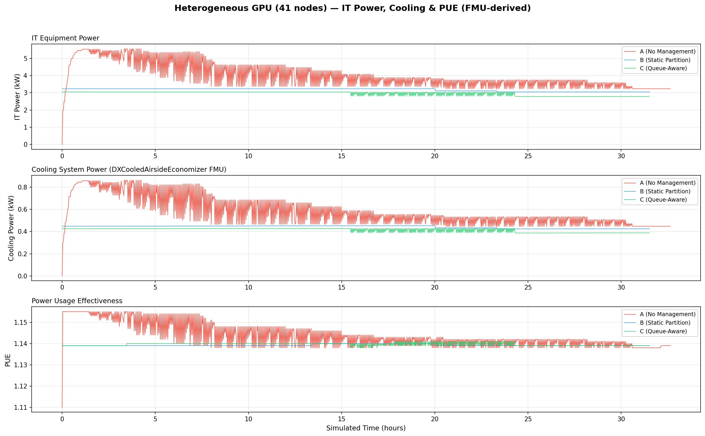
Three-panel stacked timeseries showing IT equipment power (kW), cooling system power (kW), and PUE over simulated time. Cooling power is computed by the DXCooledAirsideEconomizer FMU.
Facility power breakdown
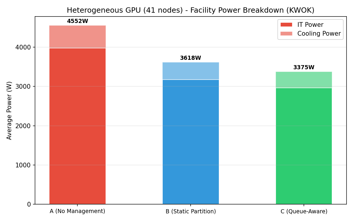
Stacked bar chart showing IT power + cooling power per baseline.
Interpretation
Why does Joulie save energy on heterogeneous GPU clusters?
- Combined CPU + GPU capping: Both CPU and GPU eco caps contribute to power savings.
- High cluster utilization (76.9% CPU): ensures eco caps engage on most nodes.
- Scheduler extender routing: performance-sensitive jobs (25%) routed to uncapped nodes, preserving throughput.
Heterogeneous challenge
The heterogeneous GPU fleet creates placement constraints: GPU jobs require specific vendor/product node selectors. This limits the operator’s flexibility to consolidate work onto performance nodes. The queue-aware policy partially mitigates this through dynamic adjustment.
Why queue-aware (C) outperforms static (B)
On a 41-node cluster, C can shift nearly all nodes to eco during low-demand periods, capturing deeper savings than B’s fixed 35% performance allocation.
Annual projections (5,000-node scale)
Extrapolating to a 5,000-node cluster (~122× the 41-node test cluster):
| Metric | B (Static Partition) | C (Queue-Aware) |
|---|---|---|
| Annual energy saved | 855 MWh | 1,085 MWh |
| Equivalent US homes powered | 81 homes | 103 homes |
| Cost savings (@ $0.10/kWh) | $85,450/yr | $108,450/yr |
| CO₂ avoided (@ 0.385 kg/kWh) | 329 tonnes/yr | 418 tonnes/yr |
Assumptions: 8,760 h/yr continuous operation, $0.10/kWh, 0.385 kg CO₂/kWh (EPA US grid avg), 10,500 kWh/yr per US household (EIA).